(a.k.a. Spreads and Butterflies Part Zero)
Interest Rate Swap markets are jargon-heavy. Traders live and breathe the language. Professional investors pick-up the nuances over time and the vicious circle of incomprehensibility is complete.
However, now that Swaps markets have transitioned to electronic trading, will we see market-standard terms adopted across asset-classes? As a result, will we witness the death of the phrase “mine the snake, two yards the belly”?
Curve Trade Definition
Trading strategy; to take a view on the shape of a (Swaps) curve.
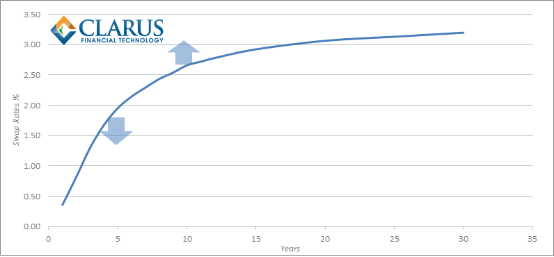
Any interest rate swap will make or lose money as Rates go up or down. But what if an investor does not have an opinion on whether rates will go up or down? Perhaps, they think that short-term rates will go down and long-term interest rates will go up. In this case, they can employ a curve trading strategy.
Spread Trade Definition
 Trading strategy; to benefit from differing movements between two instruments, through the simultaneous purchase and sale of two distinct legs.
Our investor believes that 10 year rates will move differently to 5 year rates – in which case, they would be well served to enter a curve trade. If they think 10 year rates will go up (or go up faster) they should pay the fixed rate on a 10 year swap; and if they think 5 year rates will go down (or go up slower) they should receive on a 5 year swap.
This strategy highlights a very important feature of curve trading. These trading strategies are not held to maturity. In the case of a 5 year versus 10 year position, if our investor held such a position for 5 years, they would see their 5 year swap expire and be left with one outstanding swap – i.e. their original 10 year interest rate swap will now have only 5 years until maturity. It would therefore cease to be a curve trade!
Mechanics of a Spread Trade
Price
Let \( S_{(0,t_1)} \) denote the Swap rate between \( t_0 \) and \( t_1 \) where \(t_2 > t_1\);
\(Price=S_{(0,t_2)} – S_{(0,t_1)}\)
The price of a spread trade is the yield spread between two maturities (“legs”), expressed in basis points. As a swaps curve is typically upward sloping (i.e. long swap rates are higher than short swap rates – a.k.a the term premium), it is convention to quote a spread as a positive number and calculate the price as the longest swap rate minus the shortest swap rate.
Size
Let \( D_{(0,t_1)} \) denote the DV01 of Swap \( S_{(0,t_1)} \) between \( t_0 \) and \( t_1 \); and \( N_{(0,t_1)} \) denote the Notional of Swap \( S_{(0,t_1)} \) between \( t_0 \) and \( t_1 \) where \(t_2 > t_1\) ;
\( \frac {D_{(0,t_2)}}{D_{(0,t_1)}} N_{(0,t_2)} = N_{(0,t_1)}\)
10 year interest rate swaps have a greater sensitivity to changes in interest rates than 5 year interest rate swaps (at current rates, almost double). Therefore, if we entered a swap curve trade in equal sizes of 5 year and 10 year swaps (eg $50m of each), our profit (or loss) on the package of trades would not only depend upon the yield spread between the two. If we were paying fixed on a 10 year swap, then we would also make money if swap rates moved higher, even if the spread between 5 year and 10 year swaps remained constant. Therefore, when trading a spread we agree the amount of the longest swap, and we calculate the amount of the shortest swap based upon the ratio of sensitivities (DV01s) between the two maturities. The sum of the two DV01s (the “delta”) will be zero, hence curve trading is a “delta-neutral” strategy.
Coupons
Let \( P_{(t_1,t_2)} \) denote the spread price between \( t_1 \) and \( t_2 \);
\( S_{(0,t_2)} – P_{(t_1,t_2)} = S_{(0,t_1)} \)
The swap rates (“coupons”) are set at prevailing market rates, and therefore each leg has a Net Present Value (NPV) of zero (this avoids any convexity complications). This is typically achieved by agreeing a market coupon for the longest swap and subtracting the spread at which the trade has been agreed.
Direction
We always talk in terms of the longest swap in the spread. Therefore, if the investor is buying (selling), paying (receiving), lifting (hitting), taking (giving) or putting on a steepener (flattener) they are paying fixed on the longest swap. And doing the opposite on the shortest leg.
Butterfly Trade Definition
 Trading strategy; to benefit from differing movements between three instruments. In swaps trading, the shortest and longest maturity legs are traded in equivalent directions; the risk of the intermediate maturity leg is equal and opposite to the sum of the other two legs.
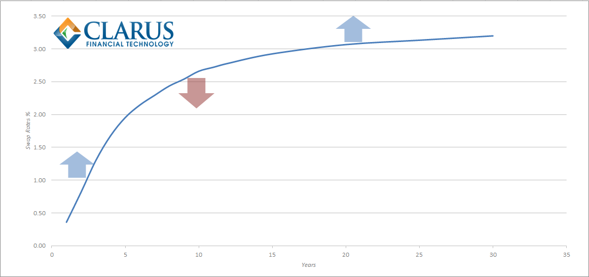
Another investor has a different view on the curve. They believe that short-term rates will head higher, medium term rates will move lower whilst long-end rates will increase. Our previous investor had a view on the slope (or steepness) of the curve; this new investor has an opinion on the shape (or curvature) of swap rates. A butterfly (or barbel) therefore involves the simultaneous trading of three maturities on the swap curve.
Mechanics of a Butterfly Trade
Price
\(Price= (2 . S_{(0,t_2)}) – S_{(0,t_1)} – S_{(0,t_3)}\); where \(t_3 > t_2 > t_1\)
A butterfly trade has three legs. The middle leg can be considered a “pivot point” which will move in the opposite direction to the short and long legs. We typically talk about the middle leg being the “belly” of the ‘fly and the other two legs called “wings”. Note that there is a double weighting for the intermediate swap rate. This is because another way to express the price of the butterfly trade is as the difference between the two spreads:
\(Price=(S_{(0,t_2)} – S_{(0,t_1)}) – (S_{(0,t_3)} – S_{(0,t_2)})\)
Size
\( \frac {D_{(0,t_2)}}{D_{(0,t_1)}} . \frac {N_{(0,t_2)}}{2} = N_{(0,t_1)}\)
We typically agree upon the size of the belly in notional terms. We use the ratio of the DV01s to then calculate the notionals of the wings. The wings are the same way round (e.g. both paying fixed); with the belly the opposite. Just as for spread trades, this is a delta-neutral curve trade, therefore the sum of the DV01s is always zero.
Coupons
We agree upon the Current Rate of \( S_{(0,t_2)} \) and one maturity spread at the time of trading.
We again try to derive current market rates such that each swap has an NPV of zero and to avoid convexity from off-market coupons. Market participants will typically agree the swap rate on the intermediate leg, plus a value for one of the tenor spreads, to imply the coupon on one of the wings. The coupon on the remaining wing is then calculated from the agreed price on the butterfly:
Let \( P_{(t_1,t_2,t_3)} \) be the Price, in %, of the butterfly.
\( S_{(0,t_1)} = (2 . S_{(0,t_2)}) – S_{(0,t_3)} – P_{(t_1,t_2,t_3)}\)
Direction
We always talk in terms of the belly swap in the ‘fly. Therefore, if the investor is buying (selling), paying (receiving), lifting (hitting), or taking (giving) a butterfly, then they are paying (receiving) fixed on the belly leg. And doing the opposite on the wings.
The Future
Recently, we have seen the democratization of data in our markets. We have a level playing field of execution. I’d like to propose we complete the demystification process and use less jargon whenever possible!
(And before anyone asks – the “snake” is market slang for a butterfly of invoice spreads traded against German government bond futures – the Schatz-Bobl-Bund versus swaps of matching maturities. And the “badger” is a 2y5y10y swap butterfly, starting in 1 years time. Craziness I tell you!)
Update 16-Oct-2014:
We received this useful feedback from Igor Hlivka
