- LIBOR transition has transformed LIBOR swap portfolios into OIS portfolios on the new RFR rates.
- Naïve valuations of seasoned swaps will be noticeably slower.
- The obscure Chilean Camara index provides inspiration for a fast valuation technique.
- The fast valuation approach can be used in actual settlement amount calculations.
OIS swaps have coupons determined by compounded daily interest rates settled every few months. The valuation of future coupons is computationally similar to the valuation of a LIBOR payment, in that the valuation involves the ratio of two discount factors associated with the start and end of the accrual period. A problem can arise on seasoned trades in the current period. A naïve implementation will, for each trade, look up fixings for each business day, and compute the compounded growth of those fixing values. This calculation potentially involving hundreds of multiplications which is much slower than simply computing the coupon amount with a single LIBOR fixing.
How might an obscure Chilean index help?
Chris has explained the basic idea in a previous post, Indices are the best way to calculate compound interest.
To relieve the computational burden of the seasoned cashflows in the portfolio, we first define the value of an index \(I\) on the valuation date \(T_0\) as \(I_{T_0}=1.0\). Then proceed backwards to form \(I_{T_{i-1}}=I_{T_{i}}(1.0+\alpha_{i-1}R(T_{i-1}, T_{i}))\), where \(R(T_{i-1}, T_{i})\) denotes the value of the fixing of the rate applying to period \(T_{i-1}\) to \(T_{i}\) and \(\alpha_{i-1}\) denotes the accrual length of the period \(T_{i-1}\) to \(T_{i}\). Then for any two accrual period dates \(T_S\) and \(T_E\) the compounded growth is just the ratio of the two associated index values; that is, $$\left((1.0+\alpha_{S}R(T_{S}, T_{S+1}))(1.0+\alpha_{S+1}R(T_{S+1}, T_{S+2}))…(1.0+\alpha_{E-1}R(T_{E-1},T_{E})\right)=\frac{I_{T_{S}}}{I_{T_{E}}}.$$ Moreover, the result is exact when the end date is the valuation date; that is, when \(T_E=T_0\) $$\left((1.0+\alpha_{S}R(T_{S}, T_{S+1}))…(1.0+\alpha_{E-1}R(T_{E-1},T_{E})\right)=I_{S}$$ since \(I_{E}=I_{T_0}=1\). This point concerning the date on which we set the index value to \(1.0\) is of no consequence to valuation and risk calculations. However, when determining actual settlement amounts it would be best if we avoid the calculation of the ratio to avoid any numerical noise entering the calculation. To that end, the date on which the index should be set to \(1.0\) would be the last maturity date of the last fixing in the OIS cashflows that settle today (which is usually at or around the valuation date). This choice avoids any numerical noise arising from the ratio of two doubles. The ability to choose this date is because our index is transient, it is only constructed in memory for the portfolio valuation on a specific day, it is not persisted like a formal published index, such as the Camara index, and so we are free to change this key date each day and recompute the index at our convenience.
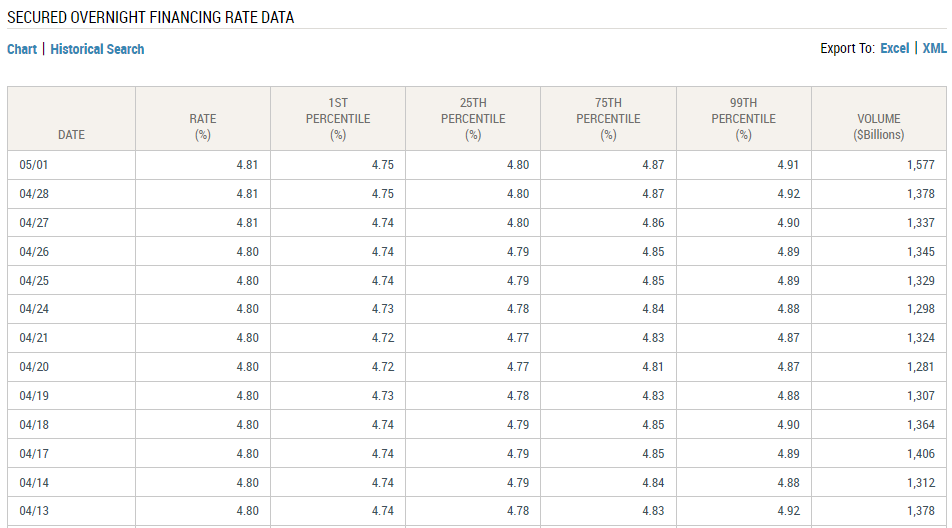
To illustrate the idea in Excel, let us consider the construction of the index for SOFR fixings on a valuation date of 2023-03-27. First we first arrange all fixings and then compute the index values, starting at a value of \(1.0\) on 2023-03-27.
Then suppose we want to compute the growth of the SOFR fixings between a short period, say, 2023-03-07 until 2023-03-14. We look up the index value on both dates (in the table we lookup the days column at 20 and 13) and find index values of 1.00255990277665 and 1.00167341198927, and the ratio is 1.00088500980137.
To validate this growth calculation, we compute the growth for each individual period, and then compute the product and we see we have the same value!
Having computed the index once, we need only look up the index values at the start and end dates of the seasoned coupons on all the OIS swaps, drastically reducing the valuation time for the portfolio and bringing it back in line with current valuation times for LIBOR swaps.
